目录

• 前言
• 一、动机和改进点
• 二、整体架构：SwinTransformer
• 三、输入设置：PatchEmbed
• 四、4个重复的Stage：BasicLayer
• • 4.1、SwinTransformerBlock
  • • 4.1.1、创建mask
    • 4.1.2、shift特征
    • 4.1.3、为shift后的特征划分窗口
    • 4.1.4、W-MSA VS SW-MSA
  • 4.2、PatchMerging
• 五、总结
• 六、一些问题
• • 6.1.为什么要W-MSA和SW-MSA混合使用？
• Reference

前言

ViT让Transformer第一次在视觉任务中暂露头角，而Swin Transfomer直接让Transformer在视觉任务中大放光彩，直接打败了当时的所有的CNN网络，一出来就直接是当时的Sota。现在的很多厉害的Transfomer变体都是Swin改进的，而且Swin Transformer这个网络在很多比赛上都会用它，分类、分割、检测基本上用它都不会差，我打的一个分类比赛就是用的它： 【记第一次kaggle比赛】PetFinder.my - Pawpularity Contest 宠物预测。当时打的时候是掉包的，两句话就创建了Model了，知其然不知所以然，这怎么行，所以今天有必要学习一下。

论文地址： https://arxiv.org/pdf/2103.14030.pdf

源码地址： https://github.com/microsoft/Swin-Transformer

这里我用的是b站大佬 霹雳吧啦Wz 改编后（相对源码作了微小改动，增加了多尺度训练）的代码：
WZMIAOMIAO

注释版本代码也同样分享到了我的Github：https://github.com/HuKai97/Classification

一、动机和改进点

VIT为了让图像可以像词向量那样输入Encoder中，而且计算量还不能太大，就直接将图像切分成一个个小的Patch，再把每个Patch当成一个词向量，把所有Patch拼接起来送入Encoder，这样当然可以降低参数量和计算量，但是当图像变大，Patch数目变多，复杂度太大。还有没有更好的输入方式了呢？

VIT主要是改变了一下图片的输入，让Transformer的Encoder可以适用于图像任务中，但是对于整个模型的架构（之前讲LN提前了），VIT是没有做什么改进的，用的还是原始的Transformer中的Encoder（整个Encoder内部各个encoder变换，但是特征的shape是不变的）。那么原始的Transformer的Encoder模块真的就适用于图像任务吗，还有没有更好的Encoder结构？

所以总结下，ViT有两个问题：

1. 尺度问题，数据集物体大大小小，但是整个Encoder过程特征尺度是不变的，效果肯定不好；
2. 划分patch，再把整张图片的所有patch都输入Encoder中，计算量太大；

所以，Swin Transformer针对这两点做出了改进：

1. Encode呈现金字塔形状。每过一个Encode图片shape变小，感受野在不停的增大，解决了尺度问题。
2. 注意力机制放在一个窗口内部。不再把整张图片的所有patch都输入Encoder，而是将各个Patch单独的输入Encoder，解决了计算量太大的问题。

二、整体架构：SwinTransformer

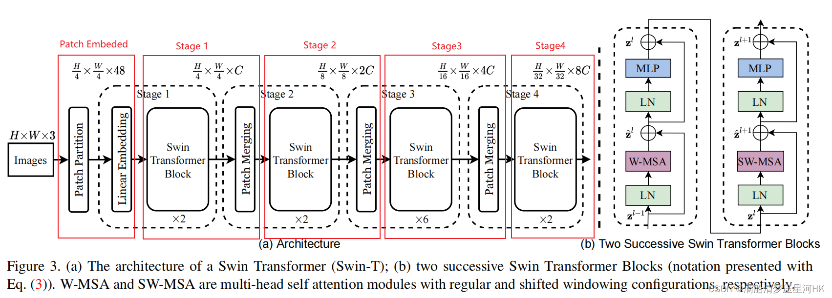
1. Patch Embeded：对输入图片 [bs，3，H_，W_] 进行处理。第一步：先经过Patch Partition，将图像划分为一个个的patch，每个patch是4x4x3大小（4x4Conv实现）得到一个 [bs，48，H_/4， W_/4] 大小的特征图；第二步：经过一个Linear Embedding层，进行Linear线性变换，得到 [bs, H_/4 * W_/4, C=96]；（但是实际代码是通过一个4x4Conv s=4实现的，其实本质还是在学习参数，一样的）
2. 经过4个stage：每个stage是若干个Swin Transformer Block + Patch Merging。前者计算相关性，后者进行采样，实现多尺度；最终经过4个stage后，特征下采样为 [bs，H_/32 * W_/32，8C=768]；
3. 分类：经过一个avgpool+flatten+Linear进行分类预测，最终得到 [bs，num_classes]；

源码：

class SwinTransformer(nn.Module):r""" Swin TransformerA PyTorch impl of : `Swin Transformer: Hierarchical Vision Transformer using Shifted Windows`  -https://arxiv.org/pdf/2103.14030"""def __init__(self, patch_size=4, in_chans=3, num_classes=1000,embed_dim=96, depths=(2, 2, 6, 2), num_heads=(3, 6, 12, 24),window_size=7, mlp_ratio=4., qkv_bias=True,drop_rate=0., attn_drop_rate=0., drop_path_rate=0.1,norm_layer=nn.LayerNorm, patch_norm=True,use_checkpoint=False, **kwargs):"""patch_size: 每个patch的大小  4x4in_chans: 输入图像的通道数 3num_classes: 分类类别数 默认1000embed_dim: 通过Linear Embedding后映射得到的通道数 也就是图片中的C 默认96depths: 每个stage中重复swin-transformer block的次数 默认(2, 2, 6, 2)num_heads: 每个stage中swin-transformer block的muti-head的个数 默认(3, 6, 12, 24)window_size: 滑动窗口的大小 默认7x7mlp_ratio: MLP中第一个全连接层Linear会将channel翻多少倍 默认4倍qkv_bias: 在muti-head self-attention中是否使用偏置 默认使用Truedrop_rate:attn_drop_rate: 在muti-head self-attention中使用的drop ratedrop_path_rate: 在每个swin-transformer block中使用的drop rate  从0慢慢增加到0.1norm_layer: LNpatch_norm:use_checkpoint: 使用可以节省内存 默认不使用"""super().__init__()self.num_classes = num_classes   # 5self.num_layers = len(depths)    # 4self.embed_dim = embed_dim       # C = 96self.patch_norm = patch_norm     # True# stage4输出特征矩阵的channelsself.num_features = int(embed_dim * 2 ** (self.num_layers - 1))   # 768 = 8Cself.mlp_ratio = mlp_ratio       # 4.0# split image into non-overlapping patchesself.patch_embed = PatchEmbed(patch_size=patch_size, in_c=in_chans, embed_dim=embed_dim,norm_layer=norm_layer if self.patch_norm else None)self.pos_drop = nn.Dropout(p=drop_rate)  # p=0# stochastic depth# [0.0, 0.00909090880304575, 0.0181818176060915, 0.027272727340459824, 0.036363635212183, 0.045454543083906174, 0.054545458406209946, 0.06363636255264282, 0.0727272778749466, 0.08181818574666977, 0.09090909361839294, 0.10000000149011612]dpr = [x.item() for x in torch.linspace(0, drop_path_rate, sum(depths))]  # stochastic depth decay rule# build layers/stages   4个self.layers = nn.ModuleList()for i_layer in range(self.num_layers):# 注意这里构建的stage和论文图中有些差异# 这里的stage不包含该stage的patch_merging层，包含的是下个stage的# stage1-3: Swin Transformer Block + Patch Merging# Stage4: Swin Transformer Blocklayers = BasicLayer(dim=int(embed_dim * 2 ** i_layer),depth=depths[i_layer],num_heads=num_heads[i_layer],window_size=window_size,mlp_ratio=self.mlp_ratio,qkv_bias=qkv_bias,drop=drop_rate,attn_drop=attn_drop_rate,drop_path=dpr[sum(depths[:i_layer]):sum(depths[:i_layer + 1])],norm_layer=norm_layer,downsample=PatchMerging if (i_layer < self.num_layers - 1) else None,use_checkpoint=use_checkpoint)self.layers.append(layers)self.norm = norm_layer(self.num_features)   # LN(768)self.avgpool = nn.AdaptiveAvgPool1d(1)self.head = nn.Linear(self.num_features, num_classes) if num_classes > 0 else nn.Identity()  # 分类头  768 -> 5self.apply(self._init_weights)   # 初始化def _init_weights(self, m):if isinstance(m, nn.Linear):nn.init.trunc_normal_(m.weight, std=.02)if isinstance(m, nn.Linear) and m.bias is not None:nn.init.constant_(m.bias, 0)elif isinstance(m, nn.LayerNorm):nn.init.constant_(m.bias, 0)nn.init.constant_(m.weight, 1.0)def forward(self, x):"""x: [bs, 3, H_, W_]"""# 1、Patch Partition + Linear Embedding# [bs, 3, H_, W_] -> [bs, H_/4 * W_/4, C] -> [bs, H_/4 * W_/4, C]   C=96x, H, W = self.patch_embed(x)  # H = H_/4  W = W_/4x = self.pos_drop(x)# 2、4 stage = 4 x (Swin Transformer Block x n + Patch Merging)# x: [bs, H_/4 * W_/4, C] -> [bs, H_/8 * W_/8, 2C] -> [bs, H_/16 * W_/16, 4C] -> [bs, H_/32 * W_/32, 8C]for layer in self.layers:x, H, W = layer(x, H, W)# 3、分类x = self.norm(x)  # LN(8C=768)x = self.avgpool(x.transpose(1, 2))  # [bs, H_/32 * W_/32, 8C] -> [bs, 8C, H_/32 * W_/32] -> [bs, 8C, 1]x = torch.flatten(x, 1)  # [bs, 8C, 1] -> [bs, 8C]x = self.head(x)  # [bs, num_classes]return x

三、输入设置：PatchEmbed

源码和论文有出入，这里直接使用一个4x4Conv s=4，实现下采样的过程。对输入图片 [bs，3，H_，W_]进行初步处理，得到一个[bs, H_/4 * W_/4, C=96]大小的特征图。源码如下：

class PatchEmbed(nn.Module):"""2D Image to Patch Embedding  [bs, 3, H_, W_] -> [B, H_/4 * W_/4, C=96]"""def __init__(self, patch_size=4, in_c=3, embed_dim=96, norm_layer=None):"""patch_size: 每个patch的大小 4x4in_c: 输入图像的channel 3embed_dim: 96 = Cnorm_layer: LN"""super().__init__()patch_size = (patch_size, patch_size)self.patch_size = patch_sizeself.in_chans = in_cself.embed_dim = embed_dimself.proj = nn.Conv2d(in_c, embed_dim, kernel_size=patch_size, stride=patch_size)  # 4x4Conv 下采样4倍 c：3->96self.norm = norm_layer(embed_dim) if norm_layer else nn.Identity()def forward(self, x):# x: [bs, 3, H_, W_]_, _, H, W = x.shape# padding# 如果输入图片的H，W不是patch_size的整数倍，需要进行paddingpad_input = (H % self.patch_size[0] != 0) or (W % self.patch_size[1] != 0)  # Falseif pad_input:# to pad the last 3 dimensions,# (W_left, W_right, H_top,H_bottom, C_front, C_back)x = F.pad(x, (0, self.patch_size[1] - W % self.patch_size[1],0, self.patch_size[0] - H % self.patch_size[0],0, 0))# 1、Patch Partition# 下采样patch_size倍  [bs, 3, H_, W_] -> [bs, C=96, H_/4, W_/4]x = self.proj(x)_, _, H, W = x.shape  # H=H_/4  W=W_/4# flatten: [B, C, H_/4, W_/4] -> [B, C, H_/4 * W_/4]# transpose: [B, C, H_/4 * W_/4] -> [B, H_/4 * W_/4, C]x = x.flatten(2).transpose(1, 2)x = self.norm(x)return x, H, W

四、4个重复的Stage：BasicLayer

每个stage都由若干个Swin Transformer Block 和 1个Patch Merging组成。

class BasicLayer(nn.Module):"""A basic Swin Transformer layer for one stage."""def __init__(self, dim, depth, num_heads, window_size,mlp_ratio=4., qkv_bias=True, drop=0., attn_drop=0.,drop_path=0., norm_layer=nn.LayerNorm, downsample=None, use_checkpoint=False):"""dim: C = 96depth: 重叠的Swin Transformer Block个数num_heads: muti-head self-transformer的头数window_size: 窗口大小7x7mlp_ratio: MLP中第一个全连接层Linear会将channel翻多少倍 默认4倍qkv_bias: 在muti-head self-attention中是否使用偏置 默认使用Truedrop: patch_embed之后一般要接一个Dropout 但是默认是 0.0attn_drop: 在muti-head self-attention中使用的drop rate  0.0drop_path: list: depth  存放这个stage中depth个transformer block的drop ratenorm_layer: LNdownsample: Pathc Merging进行下采样use_checkpoint: Whether to use checkpointing to save memory. Default: False"""super().__init__()self.dim = dimself.depth = depthself.window_size = window_sizeself.use_checkpoint = use_checkpointself.shift_size = window_size // 2  # 3# 调用depth个swin transformer blockself.blocks = nn.ModuleList([SwinTransformerBlock(dim=dim,num_heads=num_heads,window_size=window_size,shift_size=0 if (i % 2 == 0) else self.shift_size,mlp_ratio=mlp_ratio,qkv_bias=qkv_bias,drop=drop,attn_drop=attn_drop,drop_path=drop_path[i] if isinstance(drop_path, list) else drop_path,norm_layer=norm_layer)for i in range(depth)])# patch merging layerif downsample is not None:self.downsample = downsample(dim=dim, norm_layer=norm_layer)else:self.downsample = Nonedef create_mask(self, x, H, W):...def forward(self, x, H, W):# 1、depth个swin transformer block# 因为每个stage中的特征图大小是不变的，所以每个block的mask大小是相同的 所以只需要创建一次即可# [64,49,49]  64个网格  49x49每个网格中的每个位置(49个位置)对该网格中所有位置(49个位置)的注意力蒙版attn_mask = self.create_mask(x, H, W)  # [nW, Mh*Mw, Mh*Mw]for blk in self.blocks:blk.H, blk.W = H, Wif not torch.jit.is_scripting() and self.use_checkpoint:x = checkpoint.checkpoint(blk, x, attn_mask)else:# 默认执行 调用swin transformer blockx = blk(x, attn_mask)# 2、下采样 Patch Merging# 最后一个stage是None 不执行下采样if self.downsample is not None:x = self.downsample(x, H, W)H, W = (H + 1) // 2, (W + 1) // 2  # 下采样 重新计算H Wreturn x, H, W

值得注意的是创建attention mask（create_mask）的步骤，这一步是下面SW-MSA和W-MSA的关键点，下面再详细讲解。

4.1、SwinTransformerBlock

4.1.1、创建mask

在SwinTransformerBlock中，主要是负责创建attention mask，只在shift windows muti-head attention中使用，主要是告诉我们当前位置和哪些其他位置是同属于一个windows的（因为之前有一步shift window的操作），同属于一个windows的位置的mask=0，不同属于一个位置的mask=-100。

这样到后面计算出attention之后，同一个windows位置的attention + mask再softmax值是不变的，但是不同windows位置的attention + mask(-100)，再softmax值就趋近于0了。

class BasicLayer(nn.Module):"""A basic Swin Transformer layer for one stage."""...def create_mask(self, x, H, W):"""calculate attention mask for SW-MSA（shift window muti-head self-attention）以第一个stage为例x: [bs, 56x56, 96]H: 56W: 56返回attn_mask: [64,49,49] 64个网格  49x49每个网格中的每个位置(49个位置)对该网格中所有位置(49个位置)的注意力蒙版记录每个位置需要在哪些位置计算attention"""# 保证Hp和Wp是window_size的整数倍Hp = int(np.ceil(H / self.window_size)) * self.window_size   # 56Wp = int(np.ceil(W / self.window_size)) * self.window_size   # 56# 拥有和feature map一样的通道排列顺序，方便后续window_partitionimg_mask = torch.zeros((1, Hp, Wp, 1), device=x.device)  # [1, 56, 56, 1]# 对h和w先进行切片 划分为3个区域  0=(0,-7) (-7,-3) (-3,-1)h_slices = (slice(0, -self.window_size),slice(-self.window_size, -self.shift_size),slice(-self.shift_size, None))w_slices = (slice(0, -self.window_size),slice(-self.window_size, -self.shift_size),slice(-self.shift_size, None))# 对3x3=9个区域进行划分 编号 0-8cnt = 0for h in h_slices:for w in w_slices:img_mask[:, h, w, :] = cntcnt += 1# 将img_mask划分为一个个的窗口   64个7x7大小的窗口# [1,56,56,1] -> [64,7,7,1] -> [64,7,7]mask_windows = window_partition(img_mask, self.window_size)  # [nW, Mh, Mw, 1]mask_windows = mask_windows.view(-1, self.window_size * self.window_size)  # [nW, Mh*Mw]# [nW, 1, Mh*Mw] - [nW, Mh*Mw, 1] -> [nW, Mh*Mw, Mh*Mw]=[64,49,49]# 数字相同的位置代表是同一个区域  我们就是要计算同一个区域的attention  相减之后为0的区域就是我们需要计算attention的地方# 64个网格  49x49每个网格中的每个位置(49个位置)对该网格中所有位置(49个位置)的注意力蒙版attn_mask = mask_windows.unsqueeze(1) - mask_windows.unsqueeze(2)# 对于非零区域填上-100  这些区域是不需要计算attention的  所以在之后的softmax后就会为0attn_mask = attn_mask.masked_fill(attn_mask != 0, float(-100.0)).masked_fill(attn_mask == 0, float(0.0))return attn_mask

这里涉及到划分窗口的操作：

def window_partition(x, window_size: int):"""将feature map按照window_size划分成一个个没有重叠的windowArgs:x: (B, H, W, C)window_size (int): window size(M)Returns:windows: (num_windows*B, window_size, window_size, C)"""B, H, W, C = x.shape   # 1  56  56  1x = x.view(B, H // window_size, window_size, W // window_size, window_size, C)  # [1,56,56,1] -> [1,8,7,8,7,1]# permute: [B, H//Mh, Mh, W//Mw, Mw, C] -> [B, H//Mh, W//Mh, Mw, Mw, C]# view: [B, H//Mh, W//Mw, Mh, Mw, C] -> [B*num_windows, Mh, Mw, C]windows = x.permute(0, 1, 3, 2, 4, 5).contiguous().view(-1, window_size, window_size, C)  # [1,8,7,8,7,1] -> [1,8,8,7,7,1] -> [64,7,7,1]return windows

4.1.2、shift特征

class SwinTransformerBlock(nn.Module):def forward(self, x, attn_mask):# cyclic shiftif self.shift_size > 0:  # SW-MSA# 对x特征进行移动  0-shift_size列移动到最右侧   0-shift_size行移动到最下面# -的就是从上往下 从左往右  +的就是从下往上 从右往左了# 对应的attn_mask就是传入的attn_maskshifted_x = torch.roll(x, shifts=(-self.shift_size, -self.shift_size), dims=(1, 2))else:  # W-MSA  不需要移动shifted_x = xattn_mask = None

最后计算完SW-MSA后需要将shift过的特征进行还原：

		# 之前shift过windows 再还原  从下往上 从右往左 +if self.shift_size > 0:x = torch.roll(shifted_x, shifts=(self.shift_size, self.shift_size), dims=(1, 2))else:x = shifted_x

4.1.3、为shift后的特征划分窗口

		# 为shifted_x划分窗口  与attn_mask划分的窗口对应  [bs,56,56,96] -> [512,7,7,96]  8x8xbs个7x7的窗口 x 96个通道x_windows = window_partition(shifted_x, self.window_size)  # [nW*B, Mh, Mw, C]x_windows = x_windows.view(-1, self.window_size * self.window_size, C)  # [nW*B, Mh*Mw, C]=[512,49,96]

这里的划分窗口和上面mask的划分窗口一样，就不赘述。

4.1.4、W-MSA VS SW-MSA

class WindowAttention(nn.Module):r"""W-MSA/SW-MSAWindow based multi-head self attention (W-MSA) module with relative position bias.It supports both of shifted and non-shifted window."""def __init__(self, dim, window_size, num_heads, qkv_bias=True, attn_drop=0., proj_drop=0.):"""dim: C = 96window_size: 窗口大小7x7num_heads: muti-head self-transformer的头数qkv_bias: 在muti-head self-attention中是否使用偏置 默认使用Trueproj_drop: 在muti-head self-attention中使用的drop rate  0.0"""super().__init__()self.dim = dimself.window_size = window_size  # [7, 7]self.num_heads = num_headshead_dim = dim // num_headsself.scale = head_dim ** -0.5# 初始化relative_position_bias_tableself.relative_position_bias_table = nn.Parameter(torch.zeros((2 * window_size[0] - 1) * (2 * window_size[1] - 1), num_heads))  # [2*7-1 * 2*7-1, num_heads]# 1、生成绝对位置坐标索引coords_h = torch.arange(self.window_size[0])  # tensor([0, 1, 2, 3, 4, 5, 6])coords_w = torch.arange(self.window_size[1])  # tensor([0, 1, 2, 3, 4, 5, 6])# coords = torch.stack(torch.meshgrid([coords_h, coords_w], indexing="ij"))# [2, 7, 7]  7x7窗口的xy坐标coords = torch.stack(torch.meshgrid([coords_h, coords_w]))# [2, 7, 7] -> [2, 49]  第一个是所有位置的行坐标  第二个是所有位置的列坐标coords_flatten = torch.flatten(coords, 1)# 2、生成相对位置坐标索引# [2, Mh*Mw, 1] - [2, 1, Mh*Mw] -> [2, Mh*Mw, Mh*Mw]relative_coords = coords_flatten[:, :, None] - coords_flatten[:, None, :]# [2, Mh*Mw, Mh*Mw] -> [Mh*Mw, Mh*Mw, 2]relative_coords = relative_coords.permute(1, 2, 0).contiguous()# 3、将二元相对位置坐标索引转变成一元相对位置坐标索引# 原始相对位置行/列标 = -6~6 + (window_size-1) -> 0~12# 行标 + (2 * window_size - 1) -> 13~25# 这时直接把行标 + 列标 直接把2D索引转换为1D索引 就不会出现(-1,0) (0,-1) 相加都是-1 无法区分的情况了relative_coords[:, :, 0] += self.window_size[0] - 1      # 行标 + (window_size-1)relative_coords[:, :, 1] += self.window_size[1] - 1      # 列标 + (window_size-1)relative_coords[:, :, 0] *= 2 * self.window_size[1] - 1  # 行标 + (2 * window_size - 1)# [Mh*Mw, Mh*Mw, 2] -> [Mh*Mw, Mh*Mw]   行标 + 列标   直接转换为1元索引  与relative_position_bias_table一一对应relative_position_index = relative_coords.sum(-1)# 把relative_position_index放到缓存中  因为relative_position_index是固定值  不会变的  不需要修改# 我们网络训练的其实是relative_position_bias_table中的参数  我们每次循环都从relative_position_bias_table中拿对应idx的值即可self.register_buffer("relative_position_index", relative_position_index)self.qkv = nn.Linear(dim, dim * 3, bias=qkv_bias)   # 生成qkv  3倍dim = q+k+vself.attn_drop = nn.Dropout(attn_drop)             # p=0.0self.proj = nn.Linear(dim, dim)                    # linearself.proj_drop = nn.Dropout(proj_drop)             # linear dropout p=0nn.init.trunc_normal_(self.relative_position_bias_table, std=.02)  # 初始化relative_position_bias_table参数self.softmax = nn.Softmax(dim=-1)   # softmax层def forward(self, x, mask: Optional[torch.Tensor] = None):"""x: [bsx8x8, 49, 96]  bsx  8x8个7x7大小的window size  x96channelmask: W-MSA和SW-MSA交替出现 None/[8x8,49,49]  记录8x8个7x7大小的window size  中 每个位置需要和哪些位置计算attention=0的位置表示是需要计算attention的Attention(Q,K,V) = SoftMax(Q*K的转置/scale + B)*V"""B_, N, C = x.shape  # batch_size*num_windows=bsx8x8, Mh*Mw=7x7, total_embed_dim=96# 生成qkv 和vit中的一样  和原始的transformer有区别  但是本质都是相同的 都是通过学习参数把输入的x映射到3个空间上# qkv(): -> [batch_size*num_windows, Mh*Mw, 3 * total_embed_dim]# reshape: -> [batch_size*num_windows, Mh*Mw, 3, num_heads, embed_dim_per_head]# permute: -> [3, batch_size*num_windows, num_heads, Mh*Mw, embed_dim_per_head] = [3,bsx8x8,3,7x7,32]qkv = self.qkv(x).reshape(B_, N, 3, self.num_heads, C // self.num_heads).permute(2, 0, 3, 1, 4)# 分别获得q k v# [batch_size*num_windows, num_heads, Mh*Mw, embed_dim_per_head] = [bsx8x8,3,7x7,32]q, k, v = qkv.unbind(0)  # make torchscript happy (cannot use tensor as tuple)# 这里是先缩放再乘以k的转置  其实是一样的# transpose: -> [batch_size*num_windows, num_heads, embed_dim_per_head, Mh*Mw]# @: multiply -> [batch_size*num_windows, num_heads, Mh*Mw, Mh*Mw]q = q * self.scaleattn = (q @ k.transpose(-2, -1))# relative_position_bias_table.view: [Mh*Mw*Mh*Mw,nH] -> [Mh*Mw,Mh*Mw,nH]# 生成相对位置偏置：生成相对位置index + 去relative_position_bias_table中去取相应的可学习的bias参数relative_position_bias = self.relative_position_bias_table[self.relative_position_index.view(-1)].view(self.window_size[0] * self.window_size[1], self.window_size[0] * self.window_size[1], -1)relative_position_bias = relative_position_bias.permute(2, 0, 1).contiguous()  # [nH, Mh*Mw, Mh*Mw]# att + Battn = attn + relative_position_bias.unsqueeze(0)# softmax处理if mask is not None:# SW-MSA# mask: [nW, Mh*Mw, Mh*Mw]=[8x8,49,49]  记录8x8个7x7大小的window中每个位置需要和哪些位置计算attention#       =0的位置表示是需要计算attention的   不相同的区域位置是接近-100表示的nW = mask.shape[0]  # num_windows# attn.view: [batch_size, num_windows, num_heads, Mh*Mw, Mh*Mw]# mask.unsqueeze: [1, nW, 1, Mh*Mw, Mh*Mw]# 相同区域位置attn+0没有影响   不同区域位置attn+(-100)  再进行softmax   这个位置的attn就->0attn = attn.view(B_ // nW, nW, self.num_heads, N, N) + mask.unsqueeze(1).unsqueeze(0)attn = attn.view(-1, self.num_heads, N, N)attn = self.softmax(attn)else:# W-MSAattn = self.softmax(attn)attn = self.attn_drop(attn)# attn * v# @: multiply -> [batch_size*num_windows, num_heads, Mh*Mw, embed_dim_per_head]# transpose: -> [batch_size*num_windows, Mh*Mw, num_heads, embed_dim_per_head]# reshape: -> [batch_size*num_windows, Mh*Mw, total_embed_dim]x = (attn @ v).transpose(1, 2).reshape(B_, N, C)x = self.proj(x)x = self.proj_drop(x)return x

这个步骤和ViT中的其实差不多，只不过ViT是计算每个位置和所有位置的attention，而WindowAttention是按照窗口来计算每个位置和当前windows内所有位置的attention，计算量更小。

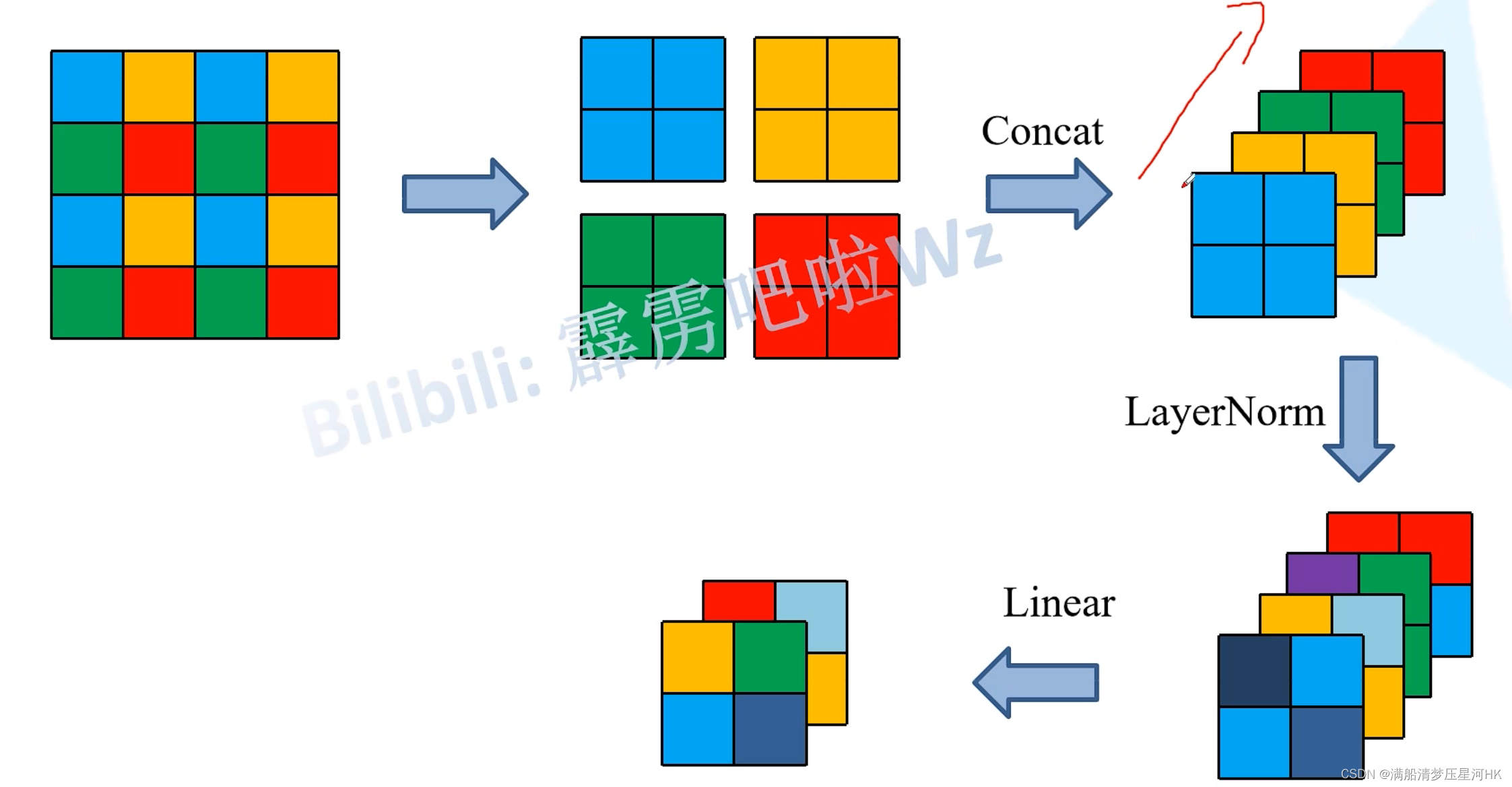
4.2、PatchMerging

这部分主要功能就是进行下采样，操作：每个一个元素取一个像素，有点类似YOLOv5中的Focus层。最后将4个特征拼接起来，再接一个Linear缩放通道。

class PatchMerging(nn.Module):r""" Patch Merging Layer. 下采样输入[bs, H_/4 * W/4, C=96]  ->  输出[bs, H_/8 * W/8, 2C] """def __init__(self, dim, norm_layer=nn.LayerNorm):super().__init__()self.dim = dim  # 输入特征的channel = 96/192/384self.reduction = nn.Linear(4 * dim, 2 * dim, bias=False)self.norm = norm_layer(4 * dim)  # LNdef forward(self, x, H, W):"""x: [bs, H_/4 * W/4, C=96]"""B, L, C = x.shape   # B=8 C=96 L= H_/4*W/4assert L == H * W, "input feature has wrong size"x = x.view(B, H, W, C)  # [bs, H_/4 * W/4, C=96] -> [bs, H_/4, W_/4, C=96]# padding# 如果输入feature map的H，W不是2的整数倍，需要进行paddingpad_input = (H % 2 == 1) or (W % 2 == 1)  # Falseif pad_input:  # 跳过# to pad the last 3 dimensions, starting from the last dimension and moving forward.# (C_front, C_back, W_left, W_right, H_top, H_bottom)# 注意这里的Tensor通道是[B, H, W, C]，所以会和官方文档有些不同x = F.pad(x, (0, 0, 0, W % 2, 0, H % 2))# 每隔一个像素取一个元素 有点像yolov5的focus层 最后一个特征 -> 4个下采样的特征# [bs, H_/4, W_/4, C=96]  ->  4 x [bs, H_/8, W_/8, C=96]x0 = x[:, 0::2, 0::2, :]  x1 = x[:, 1::2, 0::2, :] x2 = x[:, 0::2, 1::2, :]  x3 = x[:, 1::2, 1::2, :]  # 4 x [bs, H_/8, W_/8, 96] -> [bs, H_/8, W_/8, 96*4] -> [bs, H_/8 * W_/8, 4*C]x = torch.cat([x0, x1, x2, x3], -1)  x = x.view(B, -1, 4 * C)  x = self.norm(x)  # LN# Linear 将通道从4C -> 2C  [bs, H_/8 * W_/8, C*4] -> [bs, H_/8 * W_/8, 2*C]x = self.reduction(x)  return x

五、总结

为了解决ViT存在的问题：

• 尺度问题：数据集物体大大小小，但是整个Encoder过程特征尺度是不变的，效果肯定不好；
• 计算量大：划分patch，再把整张图片的所有patch都输入Encoder中，计算量太大；

改进点：

• Encode呈现金字塔形状。每过一个Stage对特征进行一次下采样，感受野在不停的增大，解决了尺度问题。所以Swin-Transformer不进适合分类任务，在下游检测、分割任务可以充分利用这种多尺度信息，检测效果很好；
• 注意力机制放在一个窗口内部。不再把整张图片的所有patch都输入Encoder，而是将各个Patch单独的输入Encoder，解决了计算量太大的问题。

关于第二点改进点还有很多的细节：

• 提出Window Muti-head Self-Attention（W-MSA)：把输入特征划分为一个个的windows窗口，只计算每个位置和当前windows窗口的所有位置的相关性Attention，其他窗口的不关心，这样就大大减少了计算量了；
• W-MSA有一个问题，不同窗口完全不相关了，那不同窗口的位置之间不就没法交互了，所以作者又提出了Shift-Window Muti-head Self-Attention（SW-MSA)。
• 特征图Shift操作其实很简单，就是特征某些行列平移，但是Shift了之后就会产生更多的窗口，计算量还是增加了，作者为了解决这个问题，引入了Mask，仍然是使用原先的窗口划分方式，但是用mask记录每个位置属于哪个窗口，相同窗口的位置mask=0，不同窗口的位置mask=-100，那么最后再用计算好的attention + mask，再softmax。于是，相同窗口的attention不变，不同窗口的attention=0，完美解决所有问题；
• 作者还在WindowAttention中引入了relative_position_bias，使用Attention(Q,K,V) = SoftMax(Q*K的转置/scale + B)*V计算公式；

六、一些问题

6.1.为什么要W-MSA和SW-MSA混合使用？

我的理解：单独的W-MSA和单独的SW-MSA其实都是固定的位置窗口（SW-MSA是对固定的区域进行shift，但是如果单独只使用SW-MSA，那么不还是固定的窗口），这样使用还是会有不同窗口无法信息交互的问题，但是混合起来使用，才能真正的起到交互作用。

Reference

b站: Swin Transformer论文精读【论文精读】

b站: 12.1 Swin-Transformer网络结构详解

b站: 12.2 使用Pytorch搭建Swin-Transformer网络